Enhancing Throughput with Dynamic Batching for Machine Learning Workloads

Dynamic batching is a technique that optimizes the performance of various workloads, from machine learning model inference to database queries. By processing multiple requests simultaneously, dynamic batching enhances throughput, minimizes the repetition of tasks, and ultimately lowers costs.

To facilitate these advantages for our users, we have integrated native dynamic batching support into Modal. In the following sections, we'll illustrate how we implemented dynamic batching in a Whisper transcription use case, achieving a remarkable 2.8x increase in throughput with just a single line of code.

The source code for our implementation can be accessed here.

Understanding Batching

At its core, batching is a fundamental methodology seen across computer systems, from write coalescing in SSDs to Nagle’s algorithm for TCP. The principle is straightforward: processing a single request often demands more than half the resources of handling two requests concurrently, making resource utilization more efficient when requests are grouped together.

This efficiency is particularly pronounced within data-intensive Python applications. Machine learning models, for instance, typically run on GPUs, which excel in parallel processing. Each individual request necessitates loading the complete model weights into the GPU’s compute units. For example, when using OpenAI’s Whisper large v3 model, over six gigabytes of data must be transferred from the GPU’s memory to the compute units for every request, despite small input and output sizes.

By merging multiple requests before passing them through the model, we can load the model weights only once, significantly improving throughput. Notably, this process often does not increase the latency for individual requests because GPU inference generally faces memory bandwidth limitations rather than compute constraints. CUDA programs can leverage overlapping computations with data transfers, optimizing performance further.

For those interested in a more in-depth exploration of this topic, I recommend reading Horace He’s blog post.

Benefits of Dynamic Batching

Traditional batching approaches often wait for a predetermined number of requests to accumulate before beginning processing. This method works efficiently under controlled request rates, such as during model training on a fixed dataset. However, it can lead to unpredictable delays when requests are received sporadically, a common scenario in web services.

Dynamic batching addresses this challenge by processing batches either when a predefined batch size is reached or after a set time limit, whichever comes first. This flexibility allows for a better balance between throughput and latency, tailored to specific workload requirements.

Some specialized inference frameworks, such as vLLM for language models, provide dynamic batching implementations and even continuous batching, where responses are sent immediately upon completion without waiting for the full batch. However, these frameworks are restricted to specific models and applications.

In contrast, Modal’s dynamic batching feature offers a simpler yet more versatile option. It can be integrated into any workload that generates single responses for individual requests.

Improving Throughput and Reducing Costs

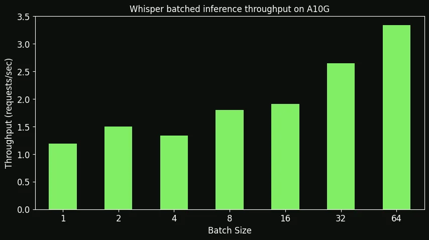
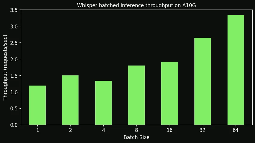
Our tests on inference with dynamic batching employed OpenAI’s Whisper large v3 model running on an A10G GPU with incremental batch sizes, up to the limits of memory capacity.

The results, showcased in a graph depicting throughput against batch size, underscores the power of dynamic batching.

Implementing dynamic batching in your model requires a straightforward modification to your inference function:

• Apply @modal.batched() with appropriate batch configuration parameters. The decorator takes max_batch_size to limit the number of inputs per batch and wait_ms to define the maximum wait time for additional inputs after the first input has been received. In our example, we chose a max_batch_size that is the largest power of 2 that doesn't exceed memory limits.
• Modify the inference function to accept lists of samples and return a list of results. In our case, both audio_samples and transcriptions are lists of equal length, and Modal automatically manages the batching of input and output.

With these adjustments, inference batching is ready to enhance your application's performance.

@app.cls(gpu="a10g")  # Configure resources in Modal as needed
class Model:
    @modal.enter()  # Model loads at startup, optimizing resource use
    def load_model(self):
        # Initialization of the model
        self.pipeline = ...

    @modal.batched(max_batch_size=64, wait_ms=1000)  # Dynamic batching configuration
    def transcribe(self, audio_samples: list) -> list:  # Accepts lists as input and output
        return self.pipeline(audio_samples, batch_size=len(audio_samples))

By setting a max_batch_size of 64, dynamic batching improved our inference throughput from approximately 1.2 requests per second to around 3.3 per container. This enhancement equated to a cost reduction of about 65% for running inference on Modal.

Are you ready to leverage dynamic batching in your application? Explore the full code example here and begin optimizing your inference processes!